通过示例学习 PyTorch

看了PyTorch提供的教程文档,里面有一个PyTorch示例,跟着做一做,顺便学习一下。

[TOC]

热身:NumPy

经过训练的三阶多项式,可以通过最小化平方的欧几里得距离来预测y = sin(x)-pipi

此实现使用 numpy 手动计算正向传播,损失和后向通过。

numpy 数组是通用的 n 维数组; 它对深度学习,梯度或计算图一无所知,而只是执行通用数值计算的一种方法。

1
2
3
4
5
6
7
8
9
10
11
12
13
14
15
16
17
18
19
20
21
22
23
24
25
26
27
28
29
30
31
32
33
34
35
36
37
38
39
40
41
42
43
44
45
import numpy as np
import math

# Create random input and output data
# 创建随机输入输出数据
x = np.linspace(-math.pi, math.pi, 2000)
y = np.sin(x)

# Randomly initialize weights
# 随机初始化权重 有四个权重
a = np.random.randn()
b = np.random.randn()
c = np.random.randn()
d = np.random.randn()
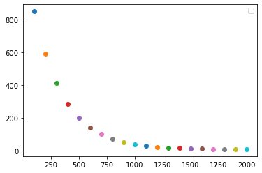
learning_rate = 1e-6 #学习率
for t in range(2000):
# Forward pass: compute predicted y
# 前向传播:计算y的值
# y = a + b x + c x^2 + d x^3
# 我在这里把它理解成泰勒展开式,展开的越多的话应该越精确
y_pred = a + b * x + c * x ** 2 + d * x ** 3

# Compute and print loss
# 计算并且输出损失 y(预测)-y(实际)之差的平方
loss = np.square(y_pred - y).sum()
if t % 100 == 99:
print(t, loss)

# Backprop to compute gradients of a, b, c, d with respect to loss
# 反向传播计算a,b,c,d相对于损失的梯度
grad_y_pred = 2.0 * (y_pred - y)
grad_a = grad_y_pred.sum()
grad_b = (grad_y_pred * x).sum()
grad_c = (grad_y_pred * x ** 2).sum()
grad_d = (grad_y_pred * x ** 3).sum()

# Update weights
# 更新权重
a -= learning_rate * grad_a
b -= learning_rate * grad_b
c -= learning_rate * grad_c
d -= learning_rate * grad_d

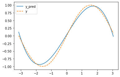
print(f'Result: y = {a} + {b} x + {c} x^2 + {d} x^3') #得出sinx的三阶多项式
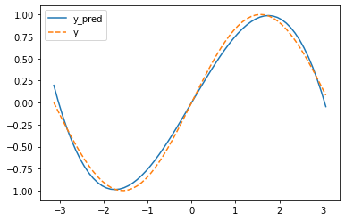
接下来绘制函数,查看差别

1
2
3
4
5
6
7
i = np.arange(-math.pi, math.pi, 0.1)
j = a + b * i + c * i ** 2 + d * i ** 3
k = np.sin(i)
plt.plot(i,j,label = "y_pred")
plt.plot(i,k,label = 'y',linestyle = '--')
plt.legend()
plt.show()

这里给出输出结果,由于存在随机数,数字可能有所差别。

1
2
3
4
5
6
7
8
9
10
11
12
13
14
15
16
17
18
19
20
21
22
0.7972626441826002 -1.798680298424662 -1.5276217691324827 2.4007340683267087
99 6770.849592635585
199 4511.314696929819
299 3008.1063132839636
399 2007.6743709025282
499 1341.5847436481672
599 897.910337306129
699 602.2501347170239
799 405.1310282453235
899 273.64401431616227
999 185.8900856790995
1099 127.29091870514203
1199 88.13752670192763
1299 61.9609647056743
1399 44.449054676909334
1499 32.725892542610765
1599 24.872466030243288
1699 19.60757126015679
1799 16.075338474872172
1899 13.703685845905285
1999 12.10998073226771
Result: y = 0.03244234711592508 + 0.8095830142635627 x + -0.005596844720483275 x^2 + -0.08662259854633106 x^3

pytorch_warmup

从图中可以看出,虽然存在一些误差,但是也大体描述了原函数图像

在这个例子中,我学习到了两点,一个是学习率,一个是梯度计算。

学习率

深度学习: 学习率 (learning rate)

Introduction

学习率 (learning rate),控制 模型的 学习进度

lrstride (步长) ,即反向传播算法中的 ηη :

ωn←ωn−η∂L∂ωnωn←ωn−η∂L∂ωn

学习率大小

学习率 大 学习率 小
学习速度
使用时间点 刚开始训练时 一定轮数过后
副作用 1,易损失值爆炸;2,易震荡 1,易过拟合;2,收敛速度慢

学习率设置

在训练过程中,一般根据训练轮数设置动态变化的学习率

  • 刚开始训练时:学习率以 0.01 ~ 0.001 为宜。
  • 一定轮数过后:逐渐减缓。
  • 接近训练结束:学习速率的衰减应该在100倍以上。

Note:
如果是 迁移学习 ,由于模型已在原始数据上收敛,此时应设置较小学习率 (≤$10^{-4}$) 在新数据上进行 微调

学习率减缓机制

轮数减缓 指数减缓 分数减缓
英文名 step decay exponential decay 1/t1/t decay
方法 每N轮学习率减半 学习率按训练轮数增长指数插值递减 lrt=lr0/(1+kt)lrt=lr0/(1+kt) ,kk 控制减缓幅度,tt 为训练轮数

把脉 目标函数损失值 曲线

理想情况下 曲线 应该是 滑梯式下降 [绿线]:

img

曲线 初始时 上扬 [红线]:

Solution:初始 学习率过大 导致 振荡,应减小学习率,并 从头 开始训练

曲线 初始时 强势下降 没多久 归于水平 [紫线]:

Solution:后期 学习率过大 导致 无法拟合,应减小学习率,并 重新训练 后几轮

曲线 全程缓慢 [黄线]:

Solution:初始 学习率过小 导致 收敛慢,应增大学习率,并 从头 开始训练

实践

根据以上学习方法,我绘制了这个程序损失函数的散点图,方便观察学习率是否合适

1
2
3
if t % 100 == 99:
print(t, loss)
plt.scatter(t,loss) # 根据损失值绘制散点图

pytorch_warmup_learningrate

图中纵轴是损失值,横轴是循环次数,可以看出这里的学习率还是比较符合要求。

计算损失梯度

这里就是损失函数的反向传播计算了,大体来说就是根据损失函数的偏导数,计算梯度下降值。(我是这么理解的,如果有错误,请帮我指正)

损失函数 $(y_{pred}-y)^2$

又有 $y_{pred}=a+bx+cx^2+dx^3$

根据链式求导原则,有
$$
\frac{\partial (y_{pred}-y)^2} {\partial a}=\frac{\partial (y_{pred}-y)^2} {\partial y_{pred}}\cdot\frac{\partial y_{pred}} {\partial a}
$$
计算出 $a=2(y_{pred}-y)$

同理可得 $b=2x(y_{pred}-y)\c=2x^2(y_{pred}-y)\d=2x^3(y_{pred}-y)$

至此,计算出了各个权值的偏导数

参考资料

深度学习: 学习率 (learning rate)

[神经网络]反向传播梯度计算数学原理


PyTorch:张量

经过训练的三阶多项式,可以通过最小化平方的欧几里得距离来预测y = sin(x)-pipi

此实现使用 PyTorch 张量手动计算正向传播,损失和后向通过。

PyTorch 张量基本上与 numpy 数组相同:它对深度学习或计算图或梯度一无所知,只是用于任意数值计算的通用 n 维数组。

numpy 数组和 PyTorch 张量之间的最大区别是 PyTorch 张量可以在 CPU 或 GPU 上运行。 要在 GPU 上运行操作,只需将张量转换为 cuda 数据类型。

1
2
3
4
5
6
7
8
9
10
11
12
13
14
15
16
17
18
19
20
21
22
23
24
25
26
27
28
29
30
31
32
33
34
35
36
37
38
39
40
41
import torch
import math

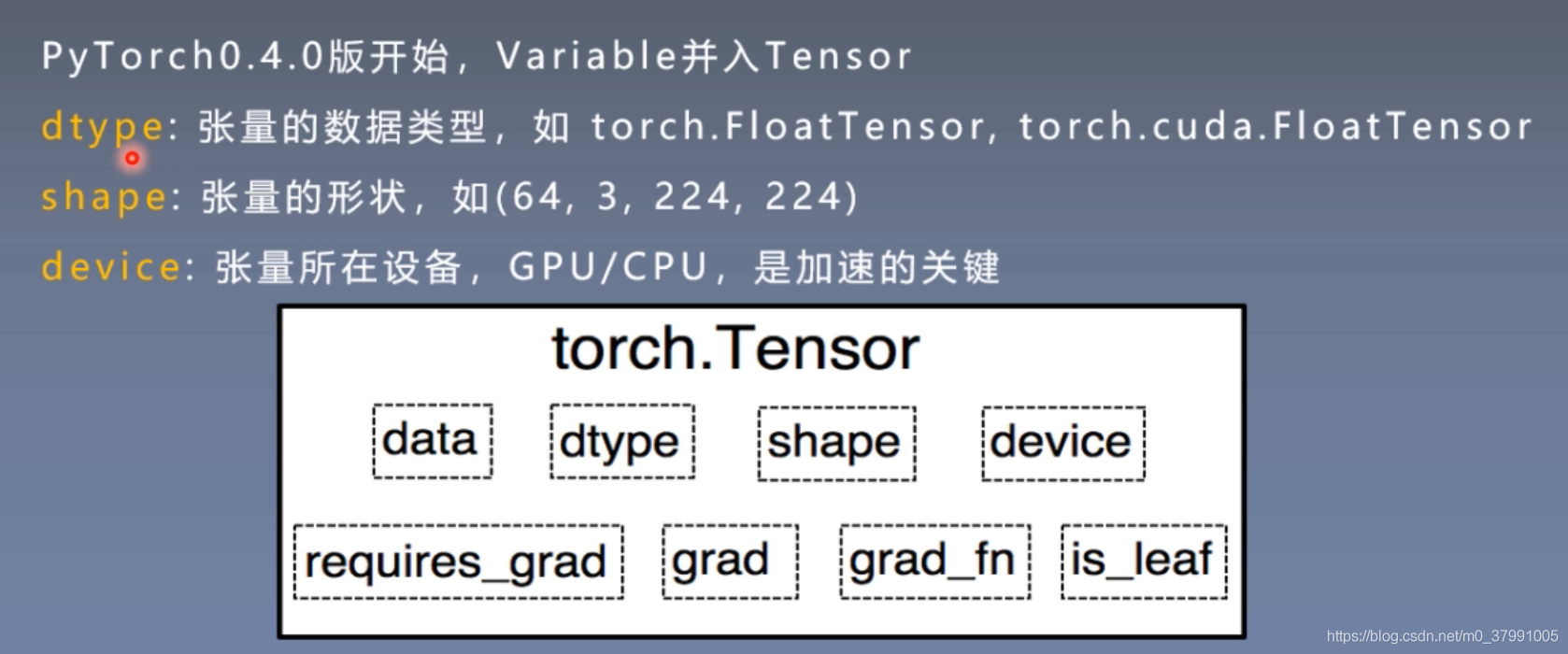
dtype = torch.float
# device = torch.device("cpu")
device = torch.device("cuda:0") # Uncomment this to run on GPU

# Create random input and output data
x = torch.linspace(-math.pi, math.pi, 2000, device=device, dtype=dtype)
y = torch.sin(x)

# Randomly initialize weights
a = torch.randn((), device=device, dtype=dtype)
b = torch.randn((), device=device, dtype=dtype)
c = torch.randn((), device=device, dtype=dtype)
d = torch.randn((), device=device, dtype=dtype)

learning_rate = 1e-6
for t in range(100000):
# Forward pass: compute predicted y
y_pred = a + b * x + c * x ** 2 + d * x ** 3

# Compute and print loss
loss = (y_pred - y).pow(2).sum().item()
if t % 100 == 99:
print(t, loss)

# Backprop to compute gradients of a, b, c, d with respect to loss
grad_y_pred = 2.0 * (y_pred - y)
grad_a = grad_y_pred.sum()
grad_b = (grad_y_pred * x).sum()
grad_c = (grad_y_pred * x ** 2).sum()
grad_d = (grad_y_pred * x ** 3).sum()

# Update weights using gradient descent
a -= learning_rate * grad_a
b -= learning_rate * grad_b
c -= learning_rate * grad_c
d -= learning_rate * grad_d

print(f'Result: y = {a.item()} + {b.item()} x + {c.item()} x^2 + {d.item()} x^3')

本次实验内容与之前相同,只是利用了PyTorch,可以在GPU上运算,语法上有些许差别。

张量

张量是什么?

张量是一个多维数组,它是标量、向量、矩阵的高维拓展。

在这里插入图片描述

张量的属性和性质

  • Variable

在这里插入图片描述

  • Tensor

Tensor 增加 3 种属性

在这里插入图片描述

Tensor attributes:

在tensor attributes中有三个类,分别为torch.dtype, torch.device, 和 torch.layout

其中, torch.dtype 是展示 torch.Tensor 数据类型的类,pytorch 有八个不同的数据类型,下表是完整的 dtype 列表.

img

Torch.device 是表现 torch.Tensor被分配的设备类型的类,其中分为’cpu’ 和 ‘cuda’两种,如果设备序号没有显示则表示此 tensor 被分配到当前设备, 比如: ‘cuda’ 等同于 ‘cuda’: X , X 为torch.cuda.current _device() 返回值

我们可以通过 tensor.device 来获取其属性,同时可以利用字符或字符+序号的方式来分配设备

1
2
3
4
5
6
7
8
9
10
11
12
13
通过字符串:
>>> torch.device('cuda:0')
device(type='cuda', index=0)
>>> torch.device('cpu')
device(type='cpu')
>>> torch.device('cuda') # 当前设备
device(type='cuda')

通过字符串和设备序号:
>>> torch.device('cuda', 0)
device(type='cuda', index=0)
>>> torch.device('cpu', 0)
device(type='cpu', index=0)

此外,cpu 和 cuda 设备的转换使用 ‘to’ 来实现:

1
2
3
4
5
>>> device_cpu = torch.device("cuda")  #声明cuda设备
>>> device_cuda = torch.device('cuda') #设备cpu设备
>>> data = torch.Tensor([1])
>>> data.to(device_cpu) #将数据转为cpu格式
>>> data.to(device_cuda) #将数据转为cuda格式

torch.layout 是表现 torch.Tensor 内存分布的类,目前只支持 torch.strided

创建tensor

  • 直接创建

torch.tensor(data, dtype=None, device=None,requires_grad=False)

data - 可以是list, tuple, numpy array, scalar或其他类型

dtype - 可以返回想要的tensor类型

device - 可以指定返回的设备

requires_grad - 可以指定是否进行记录图的操作,默认为False

需要注意的是,torch.tensor 总是会复制 data, 如果你想避免复制,可以使 torch.Tensor. detach(),如果是从 numpy 中获得数据,那么你可以用 torch.from_numpy(), 注from_numpy() 是共享内存的

1
2
3
4
5
6
7
8
9
10
11
12
13
14
15
16
17
18
>>> torch.tensor([[0.1, 1.2], [2.2, 3.1], [4.9, 5.2]])
tensor([[ 0.1000, 1.2000],
[ 2.2000, 3.1000],
[ 4.9000, 5.2000]])

>>> torch.tensor([0, 1]) # Type inference on data
tensor([ 0, 1])

>>> torch.tensor([[0.11111, 0.222222, 0.3333333]],
dtype=torch.float64,
device=torch.device('cuda:0')) # creates a torch.cuda.DoubleTensor
tensor([[ 0.1111, 0.2222, 0.3333]], dtype=torch.float64, device='cuda:0')

>>> torch.tensor(3.14159) # Create a scalar (zero-dimensional tensor)
tensor(3.1416)

>>> torch.tensor([]) # Create an empty tensor (of size (0,))
tensor([])
  • 从numpy中获得数据

torch.from_numpy(ndarry)

注:生成返回的tensor会和ndarry共享数据,任何对tensor的操作都会影响到ndarry,
反之亦然

1
2
3
4
5
6
7
>>> a = numpy.array([1, 2, 3])
>>> t = torch.from_numpy(a)
>>> t
tensor([ 1, 2, 3])
>>> t[0] = -1
>>> a
array([-1, 2, 3])
  • 创建特定的tensor

根据数值要求:

1
2
3
4
5
6
7
8
9
10
11
12
13
14
15
16
17
torch.zeros(*sizes, out=None, ..)# 返回大小为sizes的零矩阵 

torch.zeros_like(input, ..) # 返回与input相同size的零矩阵

torch.ones(*sizes, out=None, ..) #f返回大小为sizes的单位矩阵

torch.ones_like(input, ..) #返回与input相同size的单位矩阵

torch.full(size, fill_value, …) #返回大小为sizes,单位值为fill_value的矩阵

torch.full_like(input, fill_value, …) 返回与input相同size,单位值为fill_value的矩阵

torch.arange(start=0, end, step=1, …) #返回从start到end, 单位步长为step的1-d tensor.

torch.linspace(start, end, steps=100, …) #返回从start到end, 间隔中的插值数目为steps的1-d tensor

torch.logspace(start, end, steps=100, …) #返回1-d tensor ,从10^start到10^end的steps个对数间隔

根据矩阵要求:

1
2
3
4
5
torch.eye(n, m=None, out=None,…) #返回2-D 的单位对角矩阵

torch.empty(*sizes, out=None, …) #返回被未初始化的数值填充,大小为sizes的tensor

torch.empty_like(input, …) # 返回与input相同size,并被未初始化的数值填充的tensor
  • 随机采用生成:
1
2
3
4
5
6
7
8
9
10
11
12
13
14
15
torch.normal(mean, std, out=None)

torch.rand(*size, out=None, dtype=None, …) #返回[0,1]之间均匀分布的随机数值

torch.rand_like(input, dtype=None, …) #返回与input相同size的tensor, 填充均匀分布的随机数值

torch.randint(low=0, high, size,…) #返回均匀分布的[low,high]之间的整数随机值

torch.randint_like(input, low=0, high, dtype=None, …) #

torch.randn(*sizes, out=None, …) #返回大小为size,由均值为0,方差为1的正态分布的随机数值

torch.randn_like(input, dtype=None, …)

torch.randperm(n, out=None, dtype=torch.int64) # 返回0到n-1的数列的随机排列

操作tensor

基本操作:

Joining ops:

1
2
3
4
5
6
7
8
9
10
torch.cat(seq,dim=0,out=None) # 沿着dim连接seq中的tensor, 所有的tensor必须有相同的size或为empty, 其相反的操作为 torch.split() 和torch.chunk()
torch.stack(seq, dim=0, out=None) #同上

#注: .cat 和 .stack的区别在于 cat会增加现有维度的值,可以理解为续接,stack会新加增加一个维度,可以
理解为叠加
>>> a=torch.Tensor([1,2,3])
>>> torch.stack((a,a)).size()
torch.size(2,3)
>>> torch.cat((a,a)).size()
torch.size(6)
1
2
3
4
5
6
7
8
9
10
11
12
torch.gather(input, dim, index, out=None) #返回沿着dim收集的新的tensor
>> t = torch.Tensor([[1,2],[3,4]])
>> index = torch.LongTensor([[0,0],[1,0]])
>> torch.gather(t, 0, index) #由于 dim=0,所以结果为
| t[index[0, 0] 0] t[index[0, 1] 1] |
| t[index[1, 0] 0] t[index[1, 1] 1] |

对于3-D 的张量来说,可以作为

out[i][j][k] = input[index[i][j][k]][j][k] # if dim == 0
out[i][j][k] = input[i][index[i][j][k]][k] # if dim == 1
out[i][j][k] = input[i][j][index[i][j][k]] # if dim == 2

clicing ops:

1
2
3
4
5
6
7
8
9
10
torch.split(tensor, split_size_or_sections, dim=0) #将tensor 拆分成相应的组块
torch.chunk(tensor, chunks, dim=0) #将tensor 拆分成相应的组块, 最后一块会小一些如果不能整除的话#

#注:split和chunk的区别在于:
split的split_size_or_sections 表示每一个组块中的数据大小,chunks表示组块的数量
>>> a = torch.Tensor([1,2,3])
>>> torch.split(a,1)
(tensor([1.]), tensor([2.]), tensor([3.]))
>>> torch.chunk(a,1)
(tensor([ 1., 2., 3.]),)

Indexing ops:

1
2
3
4
5
6
7
8
9
10
11
12
13
14
15
torch.index_select(input, dim, index, out=None) #返回沿着dim的指定tensor, index需为longTensor类型,不共用内存

torch.masked_select(input, mask, out=None) #根据mask来返回input的值其为1-D tensor. Mask为ByteTensor, true返回,false不返回,返回值不共用内存
>>> x = torch.randn(3, 4)
>>> x
tensor([[ 0.3552, -2.3825, -0.8297, 0.3477],
[-1.2035, 1.2252, 0.5002, 0.6248],
[ 0.1307, -2.0608, 0.1244, 2.0139]])
>>> mask = x.ge(0.5)
>>> mask
tensor([[ 0, 0, 0, 0],
[ 0, 1, 1, 1],
[ 0, 0, 0, 1]], dtype=torch.uint8)
>>> torch.masked_select(x, mask)
tensor([ 1.2252, 0.5002, 0.6248, 2.0139])

Mutation ops:

1
2
3
4
5
6
7
8
9
10
11
12
13
14
15
16
17
18
19
20
21
22
23
24
25
26
27
28
29
30
31
32
33
34
torch.transpose(input, dim0, dim1, out=None) #返回dim0和dim1交换后的tensor
torch.t(input, out=None) #专为2D矩阵的转置,是transpose的便捷函数

torch.squeeze(input, dim, out=None) #默认移除所有size为1的维度,当dim指定时,移除指定size为1的维度. 返回的tensor会和input共享存储空间,所以任何一个的改变都会影响另一个
torch.unsqueeze(input, dim, out=None) #扩展input的size, 如 A x B 变为 1 x A x B

torch.reshape(input, shape) #返回size为shape具有相同数值的tensor, 注意 shape=(-1,)这种表述,-1表示任意的。
#注 reshape(-1,)
>>> a=torch.Tensor([1,2,3,4,5]) #a.size 是 torch.size(5)
>>> b=a.reshape(1,-1) #表示第一维度是1,第二维度按a的size填充满
>>> b.size()
torch.size([1,5])

torch.where(condition,x,y) #根据condition的值来相应x,y的值,true返回x的值,false返回y的值,形成新的tensor

torch.unbind(tensor, dim=0) #返回tuple 解除指定的dim的绑定,相当于按指定dim拆分
>>> a=torch.Tensor([[1,2,3],[2,3,4]])
>>> torch.unbind(a,dim=0)
(torch([1,2,3]),torch([2,3,4])) # 将一个(2,3) 分为两个(3)

torch.nonzero(input, out=None) # 返回非零值的索引, 每一行都是一个非零值的索引值
>>> torch.nonzero(torch.tensor([1, 1, 1, 0, 1]))
tensor([[ 0],
[ 1],
[ 2],
[ 4]])
>>> torch.nonzero(torch.tensor([[0.6, 0.0, 0.0, 0.0],
[0.0, 0.4, 0.0, 0.0],
[0.0, 0.0, 1.2, 0.0],
[0.0, 0.0, 0.0,-0.4]]))
tensor([[ 0, 0],
[ 1, 1],
[ 2, 2],
[ 3, 3]])

Tensor操作

  • 点对点操作

三角函数:

1
2
3
4
5
6
7
8
9
10
11
torch.abs(input, out=None)
torch.acos(input, out=None)
torch.asin(input, out=None)
torch.atan(input, out=None)
torch.atan2(input, inpu2, out=None)
torch.cos(input, out=None)
torch.cosh(input, out=None)
torch.sin(input, out=None)
torch.sinh(input, out=None)
torch.tan(input, out=None)
torch.tanh(input, out=None)

基本运算,加减乘除

1
2
3
4
5
6
7
8
Torch.add(input, value, out=None)
.add(input, value=1, other, out=None)
.addcdiv(tensor, value=1, tensor1, tensor2, out=None)
.addcmul(tensor, value=1, tensor1, tensor2, out=None)
torch.div(input, value, out=None)
.div(input, other, out=None)
torch.mul(input, value, out=None)
.mul(input, other, out=None)

对数运算:

1
2
3
4
torch.log(input, out=None)  # y_i=log_e(x_i)
torch.log1p(input, out=None) #y_i=log_e(x_i+1)
torch.log2(input, out=None) #y_i=log_2(x_i)
torch.log10(input,out=None) #y_i=log_10(x_i)

幂函数:

1
torch.pow(input, exponent, out=None)  # y_i=input^(exponent)

指数运算

1
2
torch.exp(tensor, out=None)    #y_i=e^(x_i)
torch.expm1(tensor, out=None) #y_i=e^(x_i) -1

截断函数

1
2
3
4
5
6
7
8
9
10
torch.ceil(input, out=None)   #返回向正方向取得最小整数
torch.floor(input, out=None) #返回向负方向取得最大整数

torch.round(input, out=None) #返回相邻最近的整数,四舍五入

torch.trunc(input, out=None) #返回整数部分数值
torch.frac(tensor, out=None) #返回小数部分数值

torch.fmod(input, divisor, out=None) #返回input/divisor的余数
torch.remainder(input, divisor, out=None) #同上

其他运算

1
2
3
4
5
6
7
8
9
10
11
12
13
14
15
16
17
18
torch.erf(tensor, out=None)

torch.erfinv(tensor, out=None)

torch.sigmoid(input, out=None)

torch.clamp(input, min, max out=None) #返回 input<min,则返回min, input>max,则返回max,其余返回input

torch.neg(input, out=None) #out_i=-1*(input)

torch.reciprocal(input, out=None) # out_i= 1/input_i

torch.sqrt(input, out=None) # out_i=sqrt(input_i)
torch.rsqrt(input, out=None) #out_i=1/(sqrt(input_i))

torch.sign(input, out=None) #out_i=sin(input_i) 大于0为1,小于0为-1

torch.lerp(start, end, weight, out=None)
  • 降维操作
1
2
3
4
5
6
7
8
9
10
11
12
13
14
15
16
17
18
19
20
21
torch.argmax(input, dim=None, keepdim=False) #返回最大值排序的索引值
torch.argmin(input, dim=None, keepdim=False) #返回最小值排序的索引值

torch.cumprod(input, dim, out=None) #y_i=x_1 * x_2 * x_3 *…* x_i
torch.cumsum(input, dim, out=None) #y_i=x_1 + x_2 + … + x_i

torch.dist(input, out, p=2) #返回input和out的p式距离
torch.mean() #返回平均值
torch.sum() #返回总和
torch.median(input) #返回中间值
torch.mode(input) #返回众数值
torch.unique(input, sorted=False) #返回1-D的唯一的tensor,每个数值返回一次.
>>> output = torch.unique(torch.tensor([1, 3, 2, 3], dtype=torch.long))
>>> output
tensor([ 2, 3, 1])

torch.std( #返回标准差)
torch.var() #返回方差

torch.norm(input, p=2) #返回p-norm的范式
torch.prod(input, dim, keepdim=False) #返回指定维度每一行的乘积
  • 对比操作:
1
2
3
4
5
6
7
8
9
10
11
12
13
14
15
16
17
18
19
20
21
torch.eq(input, other, out=None)  #按成员进行等式操作,相同返回1
torch.equal(tensor1, tensor2) #如果tensor1和tensor2有相同的size和elements,则为true
>>> torch.eq(torch.tensor([[1, 2], [3, 4]]), torch.tensor([[1, 1], [4, 4]]))
tensor([[ 1, 0],
[ 0, 1]], dtype=torch.uint8)
>>> torch.eq(torch.tensor([[1, 2], [3, 4]]), torch.tensor([[1, 1], [4, 4]]))
tensor([[ 1, 0],
[ 0, 1]], dtype=torch.uint8)

torch.ge(input, other, out=None) # input>= other
torch.gt(input, other, out=None) # input>other
torch.le(input, other, out=None) # input=<other
torch.lt(input, other, out=None) # input<other
torch.ne(input, other, out=None) # input != other 不等于

torch.max() # 返回最大值
torch.min() # 返回最小值
torch.isnan(tensor) #判断是否为’nan’
torch.sort(input, dim=None, descending=False, out=None) #对目标input进行排序
torch.topk(input, k, dim=None, largest=True, sorted=True, out=None) #沿着指定维度返回最大k个数值及其索引值
torch.kthvalue(input, k, dim=None, deepdim=False, out=None) #沿着指定维度返回最小k个数值及其索引值
  • 频谱操作
1
2
3
4
5
torch.fft(input, signal_ndim, normalized=False)
torch.ifft(input, signal_ndim, normalized=False)
torch.rfft(input, signal_ndim, normalized=False, onesided=True)
torch.irfft(input, signal_ndim, normalized=False, onesided=True)
torch.stft(signa, frame_length, hop, …)
  • 其他操作:
1
2
3
4
5
6
7
8
9
10
11
12
13
14
15
16
17
18
19
torch.cross(input, other, dim=-1, out=None)  #叉乘(外积)

torch.dot(tensor1, tensor2) #返回tensor1和tensor2的点乘

torch.mm(mat1, mat2, out=None) #返回矩阵mat1和mat2的乘积

torch.eig(a, eigenvectors=False, out=None) #返回矩阵a的特征值/特征向量

torch.det(A) #返回矩阵A的行列式

torch.trace(input) #返回2-d 矩阵的迹(对对角元素求和)

torch.diag(input, diagonal=0, out=None) #

torch.histc(input, bins=100, min=0, max=0, out=None) #计算input的直方图

torch.tril(input, diagonal=0, out=None) #返回矩阵的下三角矩阵,其他为0

torch.triu(input, diagonal=0, out=None) #返回矩阵的上三角矩阵,其他为0

Tips:

  • 获取python number:

由于pytorch 0.4后,python number的获取统一通过 .item()方式实现:

1
2
3
4
5
>>> a = torch.Tensor([1,2,3])
>>> a[0] #直接取索引返回的是tensor数据
tensor(1.)
>>> a[0].item() #获取python number
1
  • tensor设置

判断:

1
2
torch.is_tensor()  #如果是pytorch的tensor类型返回true
torch.is_storage() # 如果是pytorch的storage类型返回ture

这里还有一个小技巧,如果需要判断tensor是否为空,可以如下

1
2
3
4
5
>>> a=torch.Tensor()
>>> len(a)
0
>>> len(a) is 0
True

设置: 通过一些内置函数,可以实现对tensor的精度, 类型,print打印参数等进行设置

1
2
3
4
5
6
7
8
9
10
11
12
13
14
15
16
torch.set_default_dtype(d)  #对torch.tensor() 设置默认的浮点类型

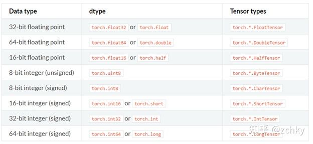
torch.set_default_tensor_type() # 同上,对torch.tensor()设置默认的tensor类型
>>> torch.tensor([1.2, 3]).dtype # initial default for floating point is torch.float32
torch.float32
>>> torch.set_default_dtype(torch.float64)
>>> torch.tensor([1.2, 3]).dtype # a new floating point tensor
torch.float64
>>> torch.set_default_tensor_type(torch.DoubleTensor)
>>> torch.tensor([1.2, 3]).dtype # a new floating point tensor
torch.float64

torch.get_default_dtype() #获得当前默认的浮点类型torch.dtype

torch.set_printoptions(precision=None, threshold=None, edgeitems=None, linewidth=None, profile=None)#)
## 设置printing的打印参数

张量的创建

1. 直接创建

1
2
3
4
5
6
7
8
torch.tensor(
data, # 数据, 可以是list, numpy
dtype=None, # 数据类型,默认与data的一致
device=None,
requires_grad=False,
pin_memory=False)

torch.from_numpy() # tensor 与原 ndarray 共享内存

2. 依据数值创建

1
2
3
4
5
6
7
8
9
10
11
12
13
14
15
16
17
18
19
20
21
22
23
24
25
26
27
28
29
30
31
32
33
34
35
36
37
38
39
40
41
42
# 依size创建全0张量
torch.zeros(*size, # size: 张量的形状, 如(3, 3)、 (3, 224,224)
out=None, # 输出的张量,和返回的张量指向同一内存地址
dtype=None,
layout=torch.strided, # 内存中布局形式, 有strided,sparse_coo等
device=None,
requires_grad=False)

# 依input形状创建全0张量
torch.zeros_like(input, # 创建与input同形状的全0张量
dtype=None,
layout=None,
device=None,
requires_grad=False)
# 全1张量,参数同上
torch.ones()
torch.ones_like()

# 依input形状创建指定数据的张量(剩余参数隐藏)
# t = torch.full((3, 3), 1)
torch.full(size, # 张量的形状, 如(3, 3)
fill_value, # 张量的值
)

# 创建等差的1维张量
torch.arange(start=0,
end,
step=1)
# 创建均分的1维张量
torch.linspace(start,
end,
steps=100) # 数列长度
# 创建对数均分的1维张量
torch.logspace(start,
end,
steps=100, # 数列长度
base=10.0) # 对数函数的底,默认为10

# 创建单位对角矩阵(2维张量)
torch.eye(n, # 矩阵行数
m=None, # 矩阵列数
)

3. 依概率分布创建张量

1
2
3
4
5
6
7
8
9
10
11
12
13
14
15
16
17
18
19
20
21
22
23
24
25
26
27
# 生成正态分布(高斯分布)
torch.normal(mean,
std,
out=None)
四种模式:
mean为标量, std为标量
mean为标量, std为张量
mean为张量, std为标量
mean为张量, std为张量

# 生成标准正态分布
torch.randn(*size) # 张量的形状
torch.randn_like()

# 在区间[0, 1)上,生成均匀分布
torch.rand(*size)
torch.rand_like()

# 区间[low, high)生成整数均匀分布
torch.randint()
torch.randint_like()

# 生成生成从0到n-1的随机排列
torch.randperm(n)

# 以input为概率,生成伯努力分布( 0-1分布,两点分布)
torch.bernoulli()

张量的操作:拼接、切分、索引和变换

张量拼接与切分

拼接

1
2
3
4
5
6
7
8
9
10
# 将张量按维度dim进行拼接
torch.cat(tensors, # 张量序列
dim=0, # 要拼接的维度
out=None)
torch.cat([torch.ones((2, 3)), torch.ones((2, 3))], dim=0) # 在第 0 维拼接,shape(4, 3)

# 在新创建的维度dim上 进行拼接
torch.stack(tensors, # 张量序列
dim=0, # 要拼接的维度
out=None)

切分

1
2
3
4
5
6
7
8
9
# 将张量按维度dim进行平均切分;返回值:张量列表
torch.chunk(input, # 要切分的张量
chunks, # 要切分的份数
dim=0) # 要切分的维度

# 将张量按维度dim进行切分;返回值:张量列表
torch.split(tensor, # 要切分的张量
split_size_or_sections, # 为int时,表示每一份的长度;为list时,按list元素切分
dim=0) # 要切分的维度

张量索引与变换

索引

1
2
3
4
5
6
7
8
9
10
# 在维度dim上,按index索引数据;返回值:依index索引数据拼接的张量
torch.index_select(input, # 要索引的张量
dim, # 要索引的维度
index, # 要索引数据的序号 torch.tensor([0, 2], dtype=torch.long)
out=None)

# 按mask中的True进行索引;返回值:一维张量
torch.masked_select(input, # 要索引的张量
mask, # 与input同形状的布尔类型张量
out=None)

变换

1
2
3
4
5
6
7
8
9
10
11
12
13
14
15
# 变换张量形状(注意事项:当张量在内存中是连续时,新张量与input共享数据内存)
torch.reshape(input,
shape)

# 交换张量的两个维度
torch.transpose(input, # 要变换的张量
dim0, # 要交换的维度
dim1) # 要交换的维度
# 2维张量转置
torch.t(input)

# 压缩长度为1的维度(轴)
torch.squeeze(input,
dim=None, # 若为None,移除所有长度为1的轴;若指定维度,当且仅当该轴长度为1时,可以被移除;
out=None)

张量数学运算

1
2
3
4
5
6
7
8
9
10
11
12
13
14
15
16
17
18
19
20
21
22
23
24
25
26
27
28
# 加减乘除
torch.add()
torch.addcdiv()
torch.addcmul()
torch.sub()
torch.div()
torch.mul()
# 对数,指数,幂函数
torch.log(input, out=None)
torch.log10(input, out=None)
torch.log2(input, out=None)
torch.exp(input, out=None)
torch.pow()
# 三角函数
torch.abs(input, out=None)
torch.acos(input, out=None)
torch.cosh(input, out=None)
torch.cos(input, out=None)
torch.asin(input, out=None)
torch.atan(input, out=None)
torch.atan2(input, other, out=None)

# 逐元素计算
# input + alpha × other
torch.add(input, # 第一个张量
alpha=1, # 乘项因子
other, # 第二个张量
out=None)

PyTorch:张量和 Autograd

经过训练的三阶多项式,可以通过最小化平方的欧几里得距离来预测y = sin(x)-pipi

此实现使用 PyTorch 张量上的运算来计算正向传播,并使用 PyTorch Autograd 来计算梯度。

PyTorch 张量表示计算图中的一个节点。 如果x是具有x.requires_grad=True的张量,则x.grad是另一个张量,其保持x相对于某个标量值的梯度。

1
2
3
4
5
6
7
8
9
10
11
12
13
14
15
16
17
18
19
20
21
22
23
24
25
26
27
28
29
30
31
32
33
34
35
36
37
38
39
40
41
42
43
44
45
46
47
48
49
50
51
52
53
54
55
56
57
58
59
60
61
62
63
import torch
import math

dtype = torch.float
device = torch.device("cpu")
# device = torch.device("cuda:0") # Uncomment this to run on GPU

# Create Tensors to hold input and outputs. 创建张量来保存输入和输出。
# By default, requires_grad=False, which indicates that we do not need to
# compute gradients with respect to these Tensors during the backward pass.
# 默认情况下,requires_grad=False,这表示我们不需要在向后传递期间计算关于这些张量的梯度。
x = torch.linspace(-math.pi, math.pi, 2000, device=device, dtype=dtype)
y = torch.sin(x)

# Create random Tensors for weights. For a third order polynomial, we need
# 4 weights: y = a + b x + c x^2 + d x^3
# 为权重创建随机张量。对于三阶多项式,我们需要4个权值:y=a+bx+cx^2+dx^3
# Setting requires_grad=True indicates that we want to compute gradients with
# respect to these Tensors during the backward pass.
# 设置requires_grad=True表示我们希望在向后传递期间计算相对于这些张量的梯度。
a = torch.randn((), device=device, dtype=dtype, requires_grad=True)
b = torch.randn((), device=device, dtype=dtype, requires_grad=True)
c = torch.randn((), device=device, dtype=dtype, requires_grad=True)
d = torch.randn((), device=device, dtype=dtype, requires_grad=True)

learning_rate = 1e-6
for t in range(2000):
# Forward pass: compute predicted y using operations on Tensors. 前向传递:使用张量运算计算预测的y。
y_pred = a + b * x + c * x ** 2 + d * x ** 3

# Compute and print loss using operations on Tensors. 使用张量运算计算并打印损耗。
# Now loss is a Tensor of shape (1,) 现在损失是一个形状的张量(1,)
# loss.item() gets the scalar value held in the loss. loss.item()获取丢失中保存的标量值。
loss = (y_pred - y).pow(2).sum()
if t % 100 == 99:
print(t, loss.item())

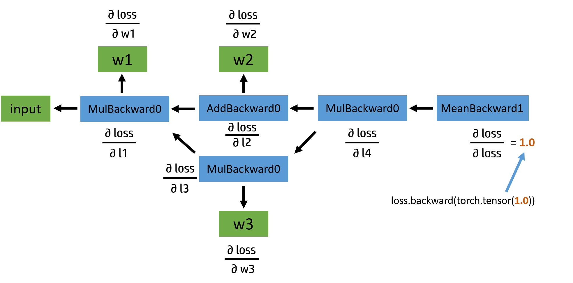
# Use autograd to compute the backward pass. This call will compute the
# gradient of loss with respect to all Tensors with requires_grad=True.
# 使用autograd计算向后传球。此调用将计算与所有张量相关的损失梯度,且requires_grad=True。
# After this call a.grad, b.grad. c.grad and d.grad will be Tensors holding
# the gradient of the loss with respect to a, b, c, d respectively.
# 在这之后调用a.grad,b.grad c.grad和d.grad将分别是关于a,b,c,d保持损失梯度的张量。
loss.backward()

# Manually update weights using gradient descent. Wrap in torch.no_grad()
# because weights have requires_grad=True, but we don't need to track this
# in autograd.
# 使用梯度下降手动更新权重。包裹火炬号()因为权重要求_grad=True,但我们不需要在autograd中跟踪它。
with torch.no_grad():
a -= learning_rate * a.grad
b -= learning_rate * b.grad
c -= learning_rate * c.grad
d -= learning_rate * d.grad

print(a.grad)
# Manually zero the gradients after updating weights 更新权重后手动将渐变归零
a.grad = None
b.grad = None
c.grad = None
d.grad = None

print(f'Result: y = {a.item()} + {b.item()} x + {c.item()} x^2 + {d.item()} x^3')

计算图

首先,我们先简单地介绍一下什么是计算图(Computational Graphs),以方便后边的讲解。假设我们有一个复杂的神经网络模型,我们把它想象成一个错综复杂的管道结构,不同的管道之间通过节点连接起来,我们有一个注水口,一个出水口。我们在入口注入数据的之后,数据就沿着设定好的管道路线缓缓流动到出水口,这时候我们就完成了一次正向传播。想象一下输入的 tensor 数据在管道中缓缓流动的场景,这就是为什么 TensorFlow 叫 TensorFlow 的原因!emmm,好像走错片场了,不过计算图在 PyTorch 中也是类似的。至于这两个非常有代表性的深度学习框架在计算图上有什么区别,我们稍后再谈。

计算图通常包含两种元素,一个是 tensor,另一个是 Function。张量 tensor 不必多说,但是大家可能对 Function 比较陌生。这里 Function 指的是在计算图中某个节点(node)所进行的运算,比如加减乘除卷积等等之类的,Function 内部有 forward()backward() 两个方法,分别应用于正向、反向传播。

1
2
3
4
a = torch.tensor(2.0, requires_grad=True)
b = a.exp()
print(b)
# tensor(7.3891, grad_fn=<ExpBackward>)

在我们做正向传播的过程中,除了执行 forward() 操作之外,还会同时会为反向传播做一些准备,为反向计算图添加 Function 节点。在上边这个例子中,变量 b 在反向传播中所需要进行的操作是 <ExpBackward>

一个具体的例子

了解了基础知识之后,现在我们来看一个具体的计算例子,并画出它的正向和反向计算图。假如我们需要计算这么一个模型:

1
2
3
4
5
l1 = input x w1
l2 = l1 + w2
l3 = l1 x w3
l4 = l2 x l3
loss = mean(l4)

这个例子比较简单,涉及的最复杂的操作是求平均,但是如果我们把其中的加法和乘法操作换成卷积,那么其实和神经网络类似。我们可以简单地画一下它的计算图:

img

下面给出了对应的代码,我们定义了inputw1w2w3 这三个变量,其中 input 不需要求导结果。根据 PyTorch 默认的求导规则,对于 l1 来说,因为有一个输入需要求导(也就是 w1 需要),所以它自己默认也需要求导,即 requires_grad=True。在整张计算图中,只有 input 一个变量是 requires_grad=False 的。正向传播过程的具体代码如下:

1
2
3
4
5
6
7
8
9
10
11
12
13
14
15
16
17
18
19
20
21
input = torch.ones([2, 2], requires_grad=False)
w1 = torch.tensor(2.0, requires_grad=True)
w2 = torch.tensor(3.0, requires_grad=True)
w3 = torch.tensor(4.0, requires_grad=True)

l1 = input * w1
l2 = l1 + w2
l3 = l1 * w3
l4 = l2 * l3
loss = l4.mean()


print(w1.data, w1.grad, w1.grad_fn)
# tensor(2.) None None

print(l1.data, l1.grad, l1.grad_fn)
# tensor([[2., 2.],
# [2., 2.]]) None <MulBackward0 object at 0x000001EBE79E6AC8>

print(loss.data, loss.grad, loss.grad_fn)
# tensor(40.) None <MeanBackward0 object at 0x000001EBE79D8208>

正向传播的结果基本符合我们的预期。我们可以看到,变量 l1grad_fn 储存着乘法操作符 <MulBackward0>,用于在反向传播中指导导数的计算。而 w1 是用户自己定义的,不是通过计算得来的,所以其 grad_fn 为空;同时因为还没有进行反向传播,grad 的值也为空。接下来,我们看一下如果要继续进行反向传播,计算图应该是什么样子:

img

反向图也比较简单,从 loss 这个变量开始,通过链式法则,依次计算出各部分的导数。说到这里,我们不妨先自己手动推导一下求导的结果,再与程序运行结果作对比。如果对这部分不感兴趣的读者,可以直接跳过。

再摆一下公式:

1
2
3
4
5
6
7
8
9
10
input = [1.0, 1.0, 1.0, 1.0]
w1 = [2.0, 2.0, 2.0, 2.0]
w2 = [3.0, 3.0, 3.0, 3.0]
w3 = [4.0, 4.0, 4.0, 4.0]

l1 = input x w1 = [2.0, 2.0, 2.0, 2.0]
l2 = l1 + w2 = [5.0, 5.0, 5.0, 5.0]
l3 = l1 x w3 = [8.0, 8.0, 8.0, 8.0]
l4 = l2 x l3 = [40.0, 40.0, 40.0, 40.0]
loss = mean(l4) = 40.0

image-20210420220025404

其他的导数计算基本上都类似,因为过程太多,这里就不全写出来了,如果有兴趣的话大家不妨自己继续算一下。

接下来我们继续运行代码,并检查一下结果和自己算的是否一致:

1
2
3
4
5
6
loss.backward()

print(w1.grad, w2.grad, w3.grad)
# tensor(28.) tensor(8.) tensor(10.)
print(l1.grad, l2.grad, l3.grad, l4.grad, loss.grad)
# None None None None None

首先我们需要注意一下的是,在之前写程序的时候我们给定的 w 们都是一个常数,利用了广播的机制实现和常数和矩阵的加法乘法,比如 w2 + l1,实际上我们的程序会自动把 w2 扩展成 [[3.0, 3.0], [3.0, 3.0]],和 l1 的形状一样之后,再进行加法计算,计算的导数结果实际上为 [[2.0, 2.0], [2.0, 2.0]],为了对应常数输入,所以最后 w2 的梯度返回为矩阵之和 8 。另外还有一个问题,虽然 w 开头的那些和我们的计算结果相符,但是为什么 l1l2l3,甚至其他的部分的求导结果都为空呢?想要解答这个问题,我们得明白什么是叶子张量。

叶子张量

对于任意一个张量来说,我们可以用 tensor.is_leaf 来判断它是否是叶子张量(leaf tensor)。在反向传播过程中,只有 is_leaf=True 的时候,需要求导的张量的导数结果才会被最后保留下来。

对于 requires_grad=False 的 tensor 来说,我们约定俗成地把它们归为叶子张量。但其实无论如何划分都没有影响,因为张量的 is_leaf 属性只有在需要求导的时候才有意义。

我们真正需要注意的是当 requires_grad=True 的时候,如何判断是否是叶子张量:当这个 tensor 是用户创建的时候,它是一个叶子节点,当这个 tensor 是由其他运算操作产生的时候,它就不是一个叶子节点。我们来看个例子:

1
2
3
4
5
6
7
8
a = torch.ones([2, 2], requires_grad=True)
print(a.is_leaf)
# True

b = a + 2
print(b.is_leaf)
# False
# 因为 b 不是用户创建的,是通过计算生成的

这时有同学可能会问了,为什么要搞出这么个叶子张量的概念出来?原因是为了节省内存(或显存)。我们来想一下,那些非叶子结点,是通过用户所定义的叶子节点的一系列运算生成的,也就是这些非叶子节点都是中间变量,一般情况下,用户不会去使用这些中间变量的导数,所以为了节省内存,它们在用完之后就被释放了。

我们回头看一下之前的反向传播计算图,在图中的叶子节点我用绿色标出了。可以看出来,被叫做叶子,可能是因为游离在主干之外,没有子节点,因为它们都是被用户创建的,不是通过其他节点生成。对于叶子节点来说,它们的 grad_fn 属性都为空;而对于非叶子结点来说,因为它们是通过一些操作生成的,所以它们的 grad_fn 不为空。

我们有办法保留中间变量的导数吗?当然有,通过使用 tensor.retain_grad() 就可以:

1
2
3
4
5
6
7
8
9
10
11
12
13
14
15
16
17
18
# 和前边一样
# ...
loss = l4.mean()

l1.retain_grad()
l4.retain_grad()
loss.retain_grad()

loss.backward()

print(loss.grad)
# tensor(1.)
print(l4.grad)
# tensor([[0.2500, 0.2500],
# [0.2500, 0.2500]])
print(l1.grad)
# tensor([[7., 7.],
# [7., 7.]])

如果我们只是想进行 debug,只需要输出中间变量的导数信息,而不需要保存它们,我们还可以使用 tensor.register_hook,例子如下:

1
2
3
4
5
6
7
8
9
10
11
12
13
14
15
16
17
18
19
# 和前边一样
# ...
loss = l4.mean()

l1.register_hook(lambda grad: print('l1 grad: ', grad))
l4.register_hook(lambda grad: print('l4 grad: ', grad))
loss.register_hook(lambda grad: print('loss grad: ', grad))

loss.backward()

# loss grad: tensor(1.)
# l4 grad: tensor([[0.2500, 0.2500],
# [0.2500, 0.2500]])
# l1 grad: tensor([[7., 7.],
# [7., 7.]])

print(loss.grad)
# None
# loss 的 grad 在 print 完之后就被清除掉了

这个函数的功能远远不止打印导数信息用以 debug,但是一般很少用,所以这里就不扩展了,更多请参考知乎提问 pytorch中的钩子(Hook)有何作用?

到此为止,我们已经讨论完了这个实例中的正向传播和反向传播的有关内容了。回过头来看, input 其实很像神经网络输入的图像,w1, w2, w3 则类似卷积核的参数,而 l1, l2, l3, l4 可以表示4个卷积层输出,如果我们把节点上的加法乘法换成卷积操作的话。实际上这个简单的模型,很像我们平时的神经网络的简化版,通过这个例子,相信大家多少也能对神经网络的正向和反向传播过程有个大致的了解了吧。

inplace 操作

现在我们来看一下本篇的重点,inplace operation。可以说,我们求导时候大部分的 bug,都出在使用了 inplace 操作上。现在我们以 PyTorch 不同的报错信息作为驱动,来讲一讲 inplace 操作吧。第一个报错信息:

1
RuntimeError: one of the variables needed for gradient computation has been modified by an inplace operation: balabala...

不少人可能会感到很熟悉,没错,我就是其中之一。之前写代码的时候竟经常报这个错,原因是对 inplace 操作不了解。要搞清楚为什么会报错,我们先来了解一下什么是 inplace 操作:inplace 指的是在不更改变量的内存地址的情况下,直接修改变量的值。我们来看两种情况,大家觉得这两种情况哪个是 inplace 操作,哪个不是?或者两个都是 inplace?

1
2
3
4
5
# 情景 1
a = a.exp()

# 情景 2
a[0] = 10

答案是:情景1不是 inplace,类似 Python 中的 i=i+1, 而情景2是 inplace 操作,类似 i+=1。依稀记得当时做机器学习的大作业,很多人都被其中一个 i+=1i=i+1 问题给坑了好长时间。那我们来实际测试一下:

1
2
3
4
5
6
7
8
9
10
11
12
13
14
15
# 我们要用到 id() 这个函数,其返回值是对象的内存地址
# 情景 1
a = torch.tensor([3.0, 1.0])
print(id(a)) # 2112716404344
a = a.exp()
print(id(a)) # 2112715008904
# 在这个过程中 a.exp() 生成了一个新的对象,然后再让 a
# 指向它的地址,所以这不是个 inplace 操作

# 情景 2
a = torch.tensor([3.0, 1.0])
print(id(a)) # 2112716403840
a[0] = 10
print(id(a), a) # 2112716403840 tensor([10., 1.])
# inplace 操作,内存地址没变

PyTorch 是怎么检测 tensor 发生了 inplace 操作呢?答案是通过 tensor._version 来检测的。我们还是来看个例子:

1
2
3
4
5
6
7
8
9
10
a = torch.tensor([1.0, 3.0], requires_grad=True)
b = a + 2
print(b._version) # 0

loss = (b * b).mean()
b[0] = 1000.0
print(b._version) # 1

loss.backward()
# RuntimeError: one of the variables needed for gradient computation has been modified by an inplace operation ...

每次 tensor 在进行 inplace 操作时,变量 _version 就会加1,其初始值为0。在正向传播过程中,求导系统记录的 b 的 version 是0,但是在进行反向传播的过程中,求导系统发现 b 的 version 变成1了,所以就会报错了。但是还有一种特殊情况不会报错,就是反向传播求导的时候如果没用到 b 的值(比如 y=x+1, y 关于 x 的导数是1,和 x 无关),自然就不会去对比 b 前后的 version 了,所以不会报错。

上边我们所说的情况是针对非叶子节点的,对于 requires_grad=True 的叶子节点来说,要求更加严格了,甚至在叶子节点被使用之前修改它的值都不行。我们来看一个报错信息:

1
RuntimeError: leaf variable has been moved into the graph interior

这个意思通俗一点说就是你的一顿 inplace 操作把一个叶子节点变成了非叶子节点了。我们知道,非叶子节点的导数在默认情况下是不会被保存的,这样就会出问题了。举个小例子:

1
2
3
4
5
6
7
8
9
10
11
a = torch.tensor([10., 5., 2., 3.], requires_grad=True)
print(a, a.is_leaf)
# tensor([10., 5., 2., 3.], requires_grad=True) True

a[:] = 0
print(a, a.is_leaf)
# tensor([0., 0., 0., 0.], grad_fn=<CopySlices>) False

loss = (a*a).mean()
loss.backward()
# RuntimeError: leaf variable has been moved into the graph interior

我们看到,在进行对 a 的重新 inplace 赋值之后,表示了 a 是通过 copy operation 生成的,grad_fn 都有了,所以自然而然不是叶子节点了。本来是该有导数值保留的变量,现在成了导数会被自动释放的中间变量了,所以 PyTorch 就给你报错了。还有另外一种情况:

1
2
3
a = torch.tensor([10., 5., 2., 3.], requires_grad=True)
a.add_(10.) # 或者 a += 10.
# RuntimeError: a leaf Variable that requires grad has been used in an in-place operation.

这个更厉害了,不等到你调用 backward,只要你对需要求导的叶子张量使用了这些操作,马上就会报错。那是不是需要求导的叶子节点一旦被初始化赋值之后,就不能修改它们的值了呢?我们如果在某种情况下需要重新对叶子变量赋值该怎么办呢?有办法!

1
2
3
4
5
6
7
8
9
10
11
12
13
14
15
16
17
18
19
20
21
22
23
24
25
26
27
28
29
# 方法一
a = torch.tensor([10., 5., 2., 3.], requires_grad=True)
print(a, a.is_leaf, id(a))
# tensor([10., 5., 2., 3.], requires_grad=True) True 2501274822696

a.data.fill_(10.)
# 或者 a.detach().fill_(10.)
print(a, a.is_leaf, id(a))
# tensor([10., 10., 10., 10.], requires_grad=True) True 2501274822696

loss = (a*a).mean()
loss.backward()
print(a.grad)
# tensor([5., 5., 5., 5.])

# 方法二
a = torch.tensor([10., 5., 2., 3.], requires_grad=True)
print(a, a.is_leaf)
# tensor([10., 5., 2., 3.], requires_grad=True) True

with torch.no_grad():
a[:] = 10.
print(a, a.is_leaf)
# tensor([10., 10., 10., 10.], requires_grad=True) True

loss = (a*a).mean()
loss.backward()
print(a.grad)
# tensor([5., 5., 5., 5.])

修改的方法有很多种,核心就是修改那个和变量共享内存,但 requires_grad=False 的版本的值,比如通过 tensor.data 或者 tensor.detach()。我们需要注意的是,要在变量被使用之前修改,不然等计算完之后再修改,还会造成求导上的问题,会报错的。


为什么 PyTorch 的求导不支持绝大部分 inplace 操作呢?从上边我们也看出来了,因为真的很 tricky。比如有的时候在一个变量已经参与了正向传播的计算,之后它的值被修改了,在做反向传播的时候如果还需要这个变量的值的话,我们肯定不能用那个后来修改的值吧,但没修改之前的原始值已经被释放掉了,我们怎么办?一种可行的办法就是我们在 Function 做 forward 的时候每次都开辟一片空间储存当时输入变量的值,这样无论之后它们怎么修改,都不会影响了,反正我们有备份在存着。但这样有什么问题?这样会导致内存(或显存)使用量大大增加。因为我们不确定哪个变量可能之后会做 inplace 操作,所以我们每个变量在做完 forward 之后都要储存一个备份,成本太高了。除此之外,inplace operation 还可能造成很多其他求导上的问题。

总之,我们在实际写代码的过程中,没有必须要用 inplace operation 的情况,而且支持它会带来很大的性能上的牺牲,所以 PyTorch 不推荐使用 inplace 操作,当求导过程中发现有 inplace 操作影响求导正确性的时候,会采用报错的方式提醒。但这句话反过来说就是,因为只要有 inplace 操作不当就会报错,所以如果我们在程序中使用了 inplace 操作却没报错,那么说明我们最后求导的结果是正确的,没问题的。这就是我们常听见的没报错就没有问题

动态图,静态图

可能大家都听说过,PyTorch 使用的是动态图(Dynamic Computational Graphs)的方式,而 TensorFlow 使用的是静态图(Static Computational Graphs)。所以二者究竟有什么区别呢,我们本节来就来讨论这个事情。

所谓动态图,就是每次当我们搭建完一个计算图,然后在反向传播结束之后,整个计算图就在内存中被释放了。如果想再次使用的话,必须从头再搭一遍,参见下边这个例子。而以 TensorFlow 为代表的静态图,每次都先设计好计算图,需要的时候实例化这个图,然后送入各种输入,重复使用,只有当会话结束的时候创建的图才会被释放(不知道这里我对 tf.Session 的理解对不对,如果有错误希望大佬们能指正一下),就像我们之前举的那个水管的例子一样,设计好水管布局之后,需要用的时候就开始搭,搭好了就往入口加水,什么时候不需要了,再把管道都给拆了。

1
2
3
4
5
6
7
8
9
10
11
12
13
# 这是一个关于 PyTorch 是动态图的例子:
a = torch.tensor([3.0, 1.0], requires_grad=True)
b = a * a
loss = b.mean()

loss.backward() # 正常
loss.backward() # RuntimeError

# 第二次:从头再来一遍
a = torch.tensor([3.0, 1.0], requires_grad=True)
b = a * a
loss = b.mean()
loss.backward() # 正常

从描述中我们可以看到,理论上来说,静态图在效率上比动态图要高。因为首先,静态图只用构建一次,然后之后重复使用就可以了;其次静态图因为是固定不需要改变的,所以在设计完了计算图之后,可以进一步的优化,比如可以将用户原本定义的 Conv 层和 ReLU 层合并成 ConvReLU 层,提高效率。

但是,深度学习框架的速度不仅仅取决于图的类型,还很其他很多因素,比如底层代码质量,所使用的底层 BLAS 库等等等都有关。从实际测试结果来说,至少在主流的模型的训练时间上,PyTorch 有着至少不逊于静态图框架 Caffe,TensorFlow 的表现。具体对比数据可以参考 这个 GitHub 仓库

大家不要急着纠正我,我知道,我现在就说:当然,在 9102 年的今天,动态图和静态图直接的界限已经开始慢慢模糊。PyTorch 模型转成 Caffe 模型越来越方便,而 TensorFlow 也加入了一些动态图机制。

除了动态图之外,PyTorch 还有一个特性,叫 eager execution。意思就是当遇到 tensor 计算的时候,马上就回去执行计算,也就是,实际上 PyTorch 根本不会去构建正向计算图,而是遇到操作就执行。真正意义上的正向计算图是把所有的操作都添加完,构建好了之后,再运行神经网络的正向传播。

正是因为 PyTorch 的两大特性:动态图和 eager execution,所以它用起来才这么顺手,简直就和写 Python 程序一样舒服,debug 也非常方便。除此之外,我们从之前的描述也可以看出,PyTorch 十分注重占用内存(或显存)大小,没有用的空间释放很及时,可以很有效地利用有限的内存。

总结

本篇文章主要讨论了 PyTorch 的 Autograd 机制和使用 inplace 操作不当可能会导致的各种报错。在实际写代码的过程中,涉及需要求导的部分,不建议大家使用 inplace 操作。除此之外我们还比较了动态图和静态图框架,PyTorch 作为动态图框架的代表之一,对初学者非常友好,而且运行速度上不逊于静态图框架,再加上现在通过 ONNX 转换为其他框架的模型用以部署也越来越方便,我觉得是一个非常称手的深度学习工具。

参考资料

  1. PyTorch Docs: AUTOGRAD MECHANICS
  2. YouTube 英文视频:PyTorch Autograd Explained - In-depth Tutorial
  3. Inplace operation in pytorch
  4. 关于 pytorch inplace operation, 需要知道的几件事
  5. cs231n 2019 lecture 6: Hardware and Software
  6. Automatic differentiation in PyTorch
  7. Understanding how Automatic Differentiation works

PyTorch:定义新的 Autograd 函数

经过训练的三阶多项式,可以通过最小化平方的欧几里得距离来预测y = sin(x)-pipi。 而不是将多项式写为y = a + bx + cx ^ 2 + dx ^ 3,我们将多项式写为y = a + b P[3](c + dx)其中P[3](x) = 1/2 (5x ^ 3 - 3x)是三次的勒让德多项式

此实现使用 PyTorch 张量上的运算来计算正向传播,并使用 PyTorch Autograd 来计算梯度。

在此实现中,我们实现了自己的自定义 Autograd 函数来执行P'[3](x)。 通过数学,P'[3](x) = 3/2 (5x ^ 2 - 1)

1
2
3
4
5
6
7
8
9
10
11
12
13
14
15
16
17
18
19
20
21
22
23
24
25
26
27
28
29
30
31
32
33
34
35
36
37
38
39
40
41
42
43
44
45
46
47
48
49
50
51
52
53
54
55
56
57
58
59
60
61
62
63
64
65
66
67
68
69
70
71
72
73
74
75
76
77
78
79
80
81
82
83
84
85
86
87
88
89
import torch
import math


class LegendrePolynomial3(torch.autograd.Function):
"""
We can implement our own custom autograd Functions by subclassing
torch.autograd.Function and implementing the forward and backward passes
which operate on Tensors.
我们可以通过子类化实现我们自己的自定义autograd函数torch.autograd.功能实现对张量进行操作的向前和向后传球。
"""

@staticmethod
def forward(ctx, input):
"""
In the forward pass we receive a Tensor containing the input and return
a Tensor containing the output. ctx is a context object that can be used
to stash information for backward computation. You can cache arbitrary
objects for use in the backward pass using the ctx.save_for_backward method.
在向前传递中,我们接收包含输入的张量,并返回包含输出的张量。
ctx是一个上下文对象,可以用来为向后计算存储信息。可以使用ctx.save_for_backward方法。
"""
ctx.save_for_backward(input)
return 0.5 * (5 * input ** 3 - 3 * input)

@staticmethod
def backward(ctx, grad_output):
"""
In the backward pass we receive a Tensor containing the gradient of the loss
with respect to the output, and we need to compute the gradient of the loss
with respect to the input.
在后向过程中,我们接收到一个张量,其中包含了与输出有关的损耗梯度,并且我们需要计算与输入有关的损耗梯度。
"""
input, = ctx.saved_tensors
return grad_output * 1.5 * (5 * input ** 2 - 1)

dtype = torch.float
device = torch.device("cpu")
# device = torch.device("cuda:0") # Uncomment this to run on GPU

# Create Tensors to hold input and outputs.
# By default, requires_grad=False, which indicates that we do not need to
# compute gradients with respect to these Tensors during the backward pass.
x = torch.linspace(-math.pi, math.pi, 2000, device=device, dtype=dtype)
y = torch.sin(x)

# Create random Tensors for weights. For this example, we need
# 4 weights: y = a + b * P3(c + d * x), these weights need to be initialized
# not too far from the correct result to ensure convergence.
# 为权重创建随机张量。对于这个例子,我们需要4个权值:y=a+b*P3(c+d*x),这些权值需要在离正确结果不太远的地方初始化以确保收敛。
# Setting requires_grad=True indicates that we want to compute gradients with
# respect to these Tensors during the backward pass.
# 设置requires_grad=True表示我们希望在向后传递期间计算相对于这些张量的梯度。
a = torch.full((), 0.0, device=device, dtype=dtype, requires_grad=True)
b = torch.full((), -1.0, device=device, dtype=dtype, requires_grad=True)
c = torch.full((), 0.0, device=device, dtype=dtype, requires_grad=True)
d = torch.full((), 0.3, device=device, dtype=dtype, requires_grad=True)

learning_rate = 5e-6
for t in range(2000):
# To apply our Function, we use Function.apply method. We alias this as 'P3'.
P3 = LegendrePolynomial3.apply

# Forward pass: compute predicted y using operations; we compute
# P3 using our custom autograd operation.
y_pred = a + b * P3(c + d * x)

# Compute and print loss
loss = (y_pred - y).pow(2).sum()
if t % 100 == 99:
print(t, loss.item())

# Use autograd to compute the backward pass.
loss.backward()

# Update weights using gradient descent
with torch.no_grad():
a -= learning_rate * a.grad
b -= learning_rate * b.grad
c -= learning_rate * c.grad
d -= learning_rate * d.grad

# Manually zero the gradients after updating weights
a.grad = None
b.grad = None
c.grad = None
d.grad = None

print(f'Result: y = {a.item()} + {b.item()} * P3({c.item()} + {d.item()} x)')

autograd

@staticmethod和@classmethod的用法

讲解一

一般来说,要使用某个类的方法,需要先实例化一个对象再调用方法。
而使用@staticmethod或@classmethod,就可以不需要实例化,直接类名.方法名()来调用。
这有利于组织代码,把某些应该属于某个类的函数给放到那个类里去,同时有利于命名空间的整洁。

既然@staticmethod和@classmethod都可以直接类名.方法名()来调用,那他们有什么区别呢
从它们的使用上来看,

  • @staticmethod不需要表示自身对象的self和自身类的cls参数,就跟使用函数一样。

  • @classmethod也不需要self参数,但第一个参数需要是表示自身类的cls参数。

    如果在@staticmethod中要调用到这个类的一些属性方法,只能直接类名.属性名或类名.方法名。
    而@classmethod因为持有cls参数,可以来调用类的属性,类的方法,实例化对象等,避免硬编码。
    下面上代码。

1
2
3
4
5
6
7
8
9
10
11
12
13
14
15
16
17
18
class A(object):  
bar = 1
def foo(self):
print 'foo'

@staticmethod
def static_foo():
print 'static_foo'
print A.bar

@classmethod
def class_foo(cls):
print 'class_foo'
print cls.bar
cls().foo()
###执行
A.static_foo()
A.class_foo()

输出

1
2
3
4
5
static_foo
1
class_foo
1
foo

讲解二

类中最常用的方法是实例方法, 即通过通过实例作为第一个参数的方法。
举个例子,一个基本的实例方法就向下面这个:

1
2
3
4
5
6
7
8
9
class Kls(object):
def __init__(self, data):
self.data = data
def printd(self):
print(self.data)
ik1 = Kls('arun')
ik2 = Kls('seema')
ik1.printd()
ik2.printd()

这会给出如下的输出:

1
2
arun
seema

这里写图片描述
然后看一下代码和示例图片:

  • 1,2参数传递给方法.
  • 3 self参数指向当前实例自身.
  • 4 我们不需要传递实例自身给方法,Python解释器自己会做这些操作的

如果现在我们想写一些仅仅与类交互而不是和实例交互的方法会怎么样呢? 我们可以在类外面写一个简单的方法来做这些,但是这样做就扩散了类代码的关系到类定义的外面. 如果像下面这样写就会导致以后代码维护的困难:

1
2
3
4
5
6
7
8
9
def get_no_of_instances(cls_obj):
return cls_obj.no_inst
class Kls(object):
no_inst = 0
def __init__(self):
Kls.no_inst = Kls.no_inst + 1
ik1 = Kls()
ik2 = Kls()
print(get_no_of_instances(Kls))

输出:

1
2

@classmethod
我们要写一个只在类中运行而不在实例中运行的方法. 如果我们想让方法不在实例中运行,可以这么做:

1
2
3
4
5
6
7
8
9
def iget_no_of_instance(ins_obj):
return ins_obj.__class__.no_inst
class Kls(object):
no_inst = 0
def __init__(self):
Kls.no_inst = Kls.no_inst + 1
ik1 = Kls()
ik2 = Kls()
print iget_no_of_instance(ik1)

输出

1
2

在Python2.2以后可以使用@classmethod装饰器来创建类方法.

1
2
3
4
5
6
7
8
9
10
11
class Kls(object):
no_inst = 0
def __init__(self):
Kls.no_inst = Kls.no_inst + 1
@classmethod
def get_no_of_instance(cls_obj):
return cls_obj.no_inst
ik1 = Kls()
ik2 = Kls()
print ik1.get_no_of_instance()
print Kls.get_no_of_instance()

输出:

1
2
2
2

这样的好处是: 不管这个方式是从实例调用还是从类调用,它都用第一个参数把类传递过来.
@staticmethod
经常有一些跟类有关系的功能但在运行时又不需要实例和类参与的情况下需要用到静态方法. 比如更改环境变量或者修改其他类的属性等能用到静态方法. 这种情况可以直接用函数解决, 但这样同样会扩散类内部的代码,造成维护困难.
比如这样:

1
2
3
4
5
6
7
8
9
10
11
12
13
14
15
16
IND = 'ON'
def checkind():
return (IND == 'ON')
class Kls(object):
def __init__(self,data):
self.data = data
def do_reset(self):
if checkind():
print('Reset done for:', self.data)
def set_db(self):
if checkind():
self.db = 'new db connection'
print('DB connection made for:',self.data)
ik1 = Kls(12)
ik1.do_reset()
ik1.set_db()

输出:

1
2
Reset done for: 12
DB connection made for: 12

如果使用@staticmethod就能把相关的代码放到对应的位置了.

1
2
3
4
5
6
7
8
9
10
11
12
13
14
15
16
17
IND = 'ON'
class Kls(object):
def __init__(self, data):
self.data = data
@staticmethod
def checkind():
return (IND == 'ON')
def do_reset(self):
if self.checkind():
print('Reset done for:', self.data)
def set_db(self):
if self.checkind():
self.db = 'New db connection'
print('DB connection made for: ', self.data)
ik1 = Kls(12)
ik1.do_reset()
ik1.set_db()

输出:

1
2
Reset done for: 12
DB connection made for: 12

下面这个更全面的代码和图示来展示这两种方法的不同
@staticmethod 和 @classmethod的不同

1
2
3
4
5
6
7
8
9
10
11
12
13
14
15
16
17
18
19
20
21
22
23
24
25
class Kls(object):
def __init__(self, data):
self.data = data
def printd(self):
print(self.data)
@staticmethod
def smethod(*arg):
print('Static:', arg)
@classmethod
def cmethod(*arg):
print('Class:', arg)
12345678910111234567891011
>>> ik = Kls(23)
>>> ik.printd()
23
>>> ik.smethod()
Static: ()
>>> ik.cmethod()
Class: (<class '__main__.Kls'>,)
>>> Kls.printd()
TypeError: unbound method printd() must be called with Kls instance as first argument (got nothing instead)
>>> Kls.smethod()
Static: ()
>>> Kls.cmethod()
Class: (<class '__main__.Kls'>,)

这里写图片描述

with torch.no_grad() 详解

torch.no_grad() 是一个上下文管理器,被该语句 wrap 起来的部分将不会track 梯度。

例如:

1
2
a = torch.tensor([1.1], requires_grad=True)
b = a * 2

打印b可看到其 grad_fn 为 mulbackward 表示是做的乘法。

1
2
3
4
5
b
Out[63]: tensor([2.2000], grad_fn=<MulBackward0>)

b.add_(2)
Out[64]: tensor([4.2000], grad_fn=<AddBackward0>)

可以看到不被wrap的情况下,b.grad_fn 为 addbackward 表示这个add 操作被track了

1
2
with torch.no_grad():
b.mul_(2)

在被包裹的情况下可以看到 b.grad_fn 还是为 add,mul 操作没有被 track. 但是注意,乘法操作是被执行了的。(4.2 -> 8.4)

1
2
b
Out[66]: tensor([8.4000], grad_fn=<AddBackward0>)

所以如果有不想被track的计算部分可以通过这么一个上下文管理器包裹起来。这样可以执行计算,但该计算不会在反向传播中被记录。

同时 torch.no_grad() 还可以作为一个装饰器。
比如在网络测试的函数前加上

1
2
3
@torch.no_grad()
def eval():
...

扩展:
同样还可以用 torch.set_grad_enabled()来实现不计算梯度。
例如:

1
2
3
4
def eval():
torch.set_grad_enabled(False)
... # your test code
torch.set_grad_enabled(True)

PyTorch:nn

经过训练的三阶多项式,可以通过最小化平方的欧几里得距离来预测y = sin(x)-pipi

此实现使用来自 PyTorch 的nn包来构建网络。 PyTorch Autograd 使定义计算图和获取梯度变得容易,但是原始的 Autograd 对于定义复杂的神经网络来说可能太低了。 这是nn包可以提供帮助的地方。 nn包定义了一组模块,您可以将其视为神经网络层,该神经网络层从输入产生输出并且可能具有一些可训练的权重。